Chapter 4: Geocentric Models

Easy

4E1. \(y_i \sim Normal(\mu,\sigma)\) defines the likelihood.

4E2. There are two parameters in the posterior distribution (\(\mu\) and \(\sigma\)).

4E3. \(P(\mu,\sigma|y) = \frac{\prod_i Normal(y_i|\mu, \sigma) Normal(\mu| 0, 10)Exp(\sigma|1)}{\int\int\prod_iNormal(y_1|\mu, \sigma)Normal(\mu|178,20)Exp(\sigma|1)d\mu d\sigma}\)

4E4. \(\mu_i = \alpha + \beta x_i\) is the linear model in the model definition.

4E5. There are three parameters in the posterior distribution (\(\alpha\), \(\beta\), \(sigma\)).

Medium

4M1. Simulate the prior for y.

#number of simulations to draw
n <- 1e4
#simulate the prior for mu
mu <- rnorm(n, mean = 0, sd = 10)
#simulate the prior for sigma
sigma <- rexp(n, rate = 1)
#simulate y using the simulated values for mu and sigma
prior_y <- rnorm(n, mean = mu, sd = sigma)
#plot the simulated prior
dens(prior_y)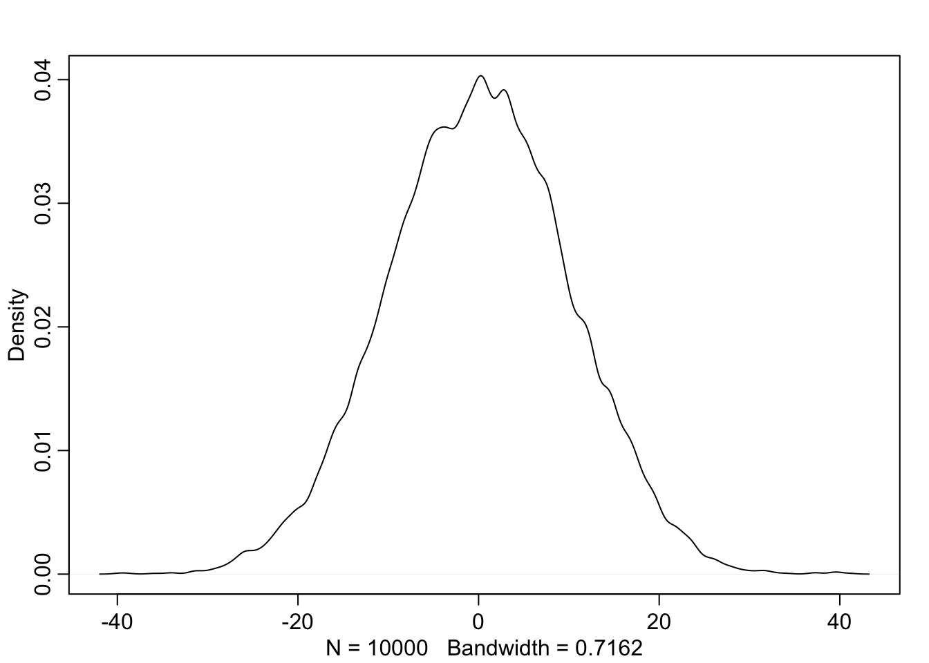

4M2.

quap(
  alist(
    y ~ dnorm(mu, sigma),
    mu ~ dnorm(0, 10), 
    sigma ~ dexp(1) 
  ))

4M3.

\[\displaylines{ y_i \sim Normal(\mu, \sigma) \\ \mu_i = \alpha + \beta X \\ \alpha \sim Normal(0, 10) \\ \beta \sim Uniform(0, 1) \\ \sigma \sim Exponential(1))} \]

4M4. Choosing Priors

#load in Howell dataset
data("Howell1")
#subset data to only look at kids
kids <- 
  Howell1 %>% 
  filter(age <= 18)
#get mean and standard deviation for priors of alpha
round(mean(kids$height),0)

## [1] 110

round(sd(kids$height),0)

## [1] 26

#kids age 10
kids_10<-
  kids %>% 
  filter(age == 10)
#kids age 16
kids_16 <-
  kids %>% 
  filter(age == 16)
#height increase per year between ages 10 and 16 assuming a steady rate
round((mean(kids_16$height) - mean(kids_10$height))/6,0)

## [1] 4

The Mathematical Model \[\displaylines{ h_i \sim Normal(\mu, \sigma)\\ \mu_i = \alpha + \beta Y \\ \alpha \sim Normal(110, 26)\\ \beta \sim Normal(4, 1.5) \\ \sigma \sim Uniform(0, 50) }\]

4M5. Assuming that height never decreases as age increases,I would change the prior on \(\beta\) from \(\beta \sim Normal(4, 1.5)\) to \(\beta \sim Log-Normal(4, 1.5)\) as a log-normal distribution enforces positive numbers.

4M6. If the variance (\(\sigma^2\)) among any age group doesn’t exceed 64cm, I would change the prior on \(\sigma\) from \(\sigma \sim Uniform(0,50)\) to \(\sigma \sim Uniform(0, \sqrt{64})\).

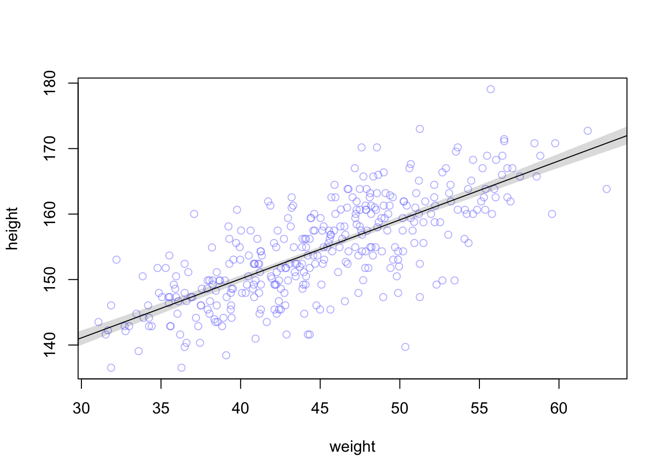
4M7.

adults <- 
  Howell1 %>% 
  filter(age >= 18)

m4.3_nomean <- quap(
  alist(
    height ~ dnorm( mu, sigma),
    mu <- a + b*weight,
    a ~ dnorm(178, 20),
    b ~ dlnorm(0, 1),
    sigma ~ dunif(0, 50)),
  data = adults)

round(vcov(m4.3),3)

##           a     b sigma
## a     0.073 0.000 0.000
## b     0.000 0.002 0.000
## sigma 0.000 0.000 0.037

round(vcov(m4.3_nomean),3)

##            a      b sigma
## a      3.601 -0.078 0.009
## b     -0.078  0.002 0.000
## sigma  0.009  0.000 0.037

There’s much more covariance when the weight isn’t centered by the mean.

## integer(0)

## integer(0)

plot_grid(original, no_mean,labels = c("m4.3", "m4.3 - no mean"), ncol = 1)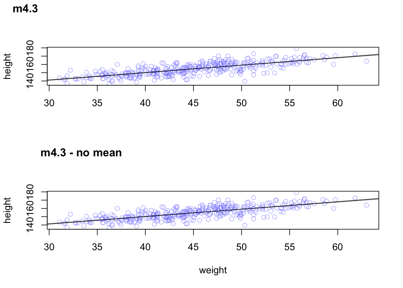

There’s no difference in the posterior predictions between the models.

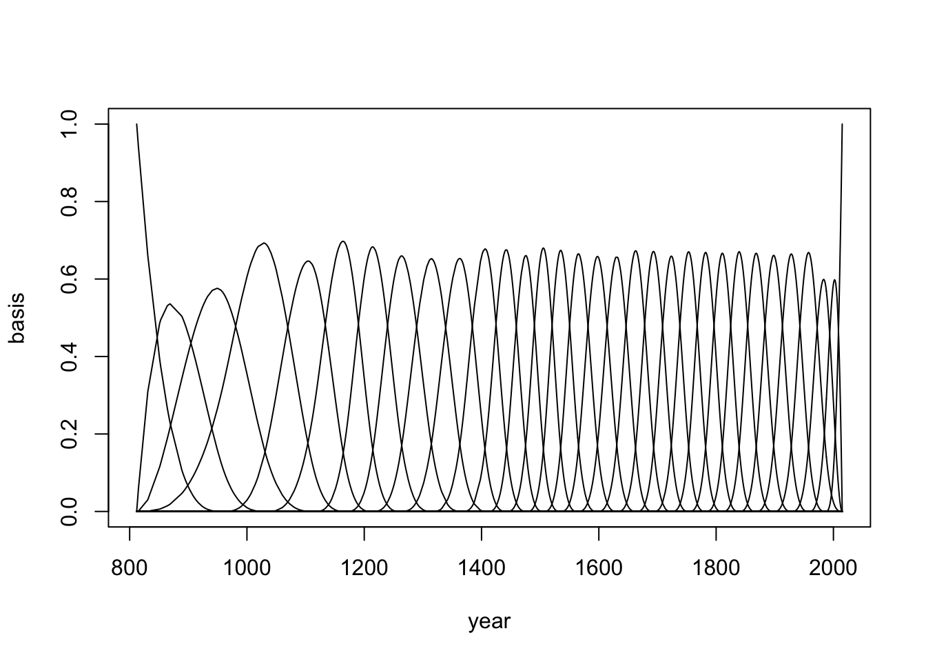
4M8.

data("cherry_blossoms")
d <- cherry_blossoms

15 Knots

20 Splines

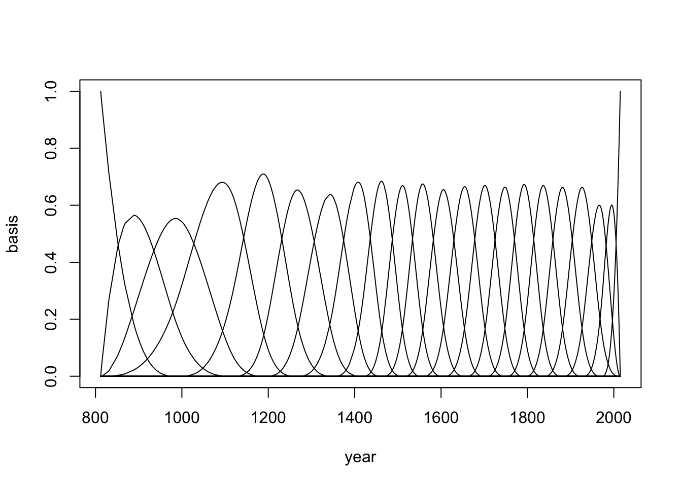__ 30 Knots__